While collecting data for a time-series analysis I quickly started running out of diskspace. While HDDs are cheap nowadays they are still not free and I’d run out of space multiple times before I get a new one at work, so I had to ask: What is the smallest, most efficient way to store all my Geotiff data?
Size matters, but so does time
In remote sensing you often have to deal with large datsets because their spatial or temporal resolution is high. A typical Landsat 8 scene clocks in at 0.7 – 1 GB and if you are trying to process satellite images for a continent or even the globe you’re easily looking at multiple terrabytes of input data. I am currently working with MODIS time series data, which will use about 4 TB of space even before any processing is done. Therefore I started looking into compression methods. One of the easiest ways to save space is by employing the compression methods some file formats and GDAL drivers support.
As an example we will use the first 7 layers of a Landsat 8 scene from central Germany (LC81940252014200LGN00). If you are working with scientific data lossy compression algorithms are out of the question to compress your input data as we don’t want to lose any information. GDAL supports three lossless compression algorithms for the GeoTiff format – Packbits, LZW and Deflate. The last two also support predictors to reduce the file size even further.
Using compression decreases the amount of space you need for your data but it will also increase the amount of time to read and write data. Depending on your situation you’ll have to use the compression method with the ideal trade-off between file size, read and write time. In my case I mostly need a reduction in space. Since I will write once but read often the read times also play an important role.
LZW, Deflate and Packbits
GDALs standard is to use no predictor for LZW and Deflate compression. Predictors store the difference in neighbouring values instead of the absolute values. If neighbouring pixels corellate this will reduce the file size even further. If not it might even increase it a bit. In other words – if your image contains smooth progression predictors might help, if it contains sudden jumps in values they might not. You can manually set the predictor to 2 for horizontal differencing or 3 for floating point. Since Landsat 8 data has no floating point values (like most satellite imagery) we will only check for horizontal differencing.
You can use the compression methods with GDALs creation options
gdal_translate -of GTiff -co “COMPRESS=LZW” -co “PREDICTOR=2” -co “TILED=YES” uncompressed.tiff LZW-pred2-compressed.tiff
In Python you can use the options as well:
dstImg = driver.Create(dstName, srcImg.RasterXSize, srcImg.RasterYSize, 1, gdal.GDT_Int32, options = [ 'COMPRESS=DEFLATE' ])
Not sure which algorithm will be the best for your data? Neither was I. I therefore wrote a small script that compares all of them to each other in regards to file size, write time and read time. This enables you to select the compression that best suits your data.
GeoTiff compression benchmark script
Just run it with a GeoTiff of your choice and compare the results:
python GTiff_compression_benchmark.py /path/to/some/Geo.tiff
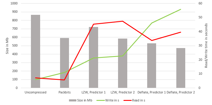
What to take away from that? Packbits is the fastest, but also offers the smallest compressions. Deflate is the smallest, slowest to write but faster to read than LZW. LZW compresses twice as fast as Deflate but is slower to decompress. In my case Deflate with horizontal differencing is the best choice, since it is the smallest and still has OK read times.
You should also consid changing your GDAL ConfigOptions. Increasing GDAL_CACHEMAX decreased my read times by about 50%.